This article outlines some of the basic concepts behind how Tensions Types and Sag are accounted for in O-Calc Pro. The full primer on this topic is linked to this article.
Any cable attached between two structures will hang between these two structures following a catenary curve. Mathematically the catenary curve is a hyperbolic curve describing the hanging cable. One can approximate the hyperbolic catenary curve with a parabolic curve. The parabolic approximation is generally within 1% of the hyperbolic formulation when the cable sag is less than 10% of the span length. The table included in the attached article for this page outlines the necessary equations for both hyperbolic and parabolic formulations. (see “Overhead Conductor Manual, 2nd Edition”, Southwire Company, 2007)
Note that the O-Calc® Pro application uses the hyperbolic formulation for the catenary curve. However, this description will use the parabolic formulation since it is easier to visualize the parabolic curves compared to the hyperbolic curves.
Catenary equations describe the relationships between the span length (distance between the structures), the cable length (the length of the cable along the curve), the cable tension, cable weight, and cable sag (how far the cable droops down in the middle between the two attachment points. These equations and the O-Calc® Pro software make a few assumptions about the properties of the cable
- There is no plastic deformation of cable due to any load or temperature changes. This implies that the linear weight of the cable is a constant.
- The load on the cable is distributed uniformly. Wind or ice build-up on the cable is uniform so that the shape of the cable remains a catenary.
-
The horizontal tension along the cable is constant.
O-Calc® Pro considers the change in conductor length (elongation) based on a number of physical parameters such as temperature changes, ice build-up on the conductors, and horizontal wind pressure blowing on the wires. This change in conductor length affects the tension of the conductor, which in turns affects the amount of sag. How O-Calc® Pro handles these various environmental effects on the conductor depends on what tension ‘mode’ the conductor is in.
O-Calc® Pro has six different modes in terms of calculating the tension and sags on each cable:
- “Tension to Sag” mode is where the user selects the initial (unloaded) tension on the cable and the program determines the mid-span final loaded tension and sag based on the cable length, tension, and loading parameters. Users typically use this method when they know what the original stringing tensions were.
- “Sag to Tension” mode is where the user selects the initial (unloaded) mid-span sag and the program determines the final (loaded) tension and final mid-span sag of the cable. The method is typically used when the mid-span sags are being measured in the field and at the nominal temperature.
- “Static” mode means that the tensions are statically determined based on a user defined percentage of the related strength of the cable. O-Calc® Pro has an option that enables the user to set the static tension percentages based on the cable type.
- “Slack” mode is the same as “Static” mode, but enables the user to set a second tension value which can be different than in the “Static Tension” value. The user can then flip-flop between the two. Note, despite the name, “Slack” mode can have any tension value, including larger than the “Static Tension” value.
- “Table” mode means that the tensions are determined by a user-created graph, wherein tension in pounds is plotted against span length in feet. The user can determine the number of points in the graph, as well as the tension to be applied at each increment of span length. The tensions between any two points on the graph are linearly interpolated between the values on the graph. O-Calc pro will then apply a static tension value as determined by the span length and table values.
- “Sag Table” mode means that the tension is calculated based on the measured sag (height difference between attachment height on the pole and span height AGL), cable weight, and loadcase; span sag in inches is plotted against span length in feet. This method enables one to model “sag to tension” mode for various span lengths.
When a cable in modeled in O-Calc® Pro in “Tension to Sag” mode, the user determines the initial (or nominal) tension and the program calculates the initial sag as well as the final tension and sag values based on the various environment loading parameters. O-Calc® Pro calls this the initial tension, but is really the tension at the nominal temperature with no wind and no ice loading, or what is referred to as “unloaded” tension. The user should enter the tension of the conductor that it has on a 60° Fahrenheit day with no wind as observed in the field.
Note, ideally the user should also consider plastic elongation of the conductor due to creep, the long-term elongation of the conductor because of various loads that have been applied to the conductor over time. In practice, taking creep into account is difficult. O-Calc® Pro enables the user to enter a ‘creep coefficient’ value for each conductor span that indicates how much plastic elongation has occurred over time, but it is difficult to get a good measure of this creep coefficient, since one needs to measure the tension value at the time the conductor was strung as well as at a later time, after a load has been applied. For these reasons, the creep coefficient in O-Calc® Pro normally is set to zero in practice. Alternatively, the user should use the tension of the conductor once it has settled due to creep.
When O-Calc® Pro applies the load case to the conductor, it will first determine the amount of elongation (increasing or decreasing) based on the temperature gradient between the nominal and current temperature using the linear thermal expansion equation:
where a is the linear expansion coefficient and is a parameter for the cable within O-Calc® Pro.
For the minimal temperature case, the conductor thermally contracts and so the sag decreases and the tension increases. Then depending on the load case applied, the amount of ice build-up is applied to the conductor as well as the horizontal wind pressure. The simulated ice build-up on the conductor as two effects: first it increases the linear weight of the conductor which causes the conductor to sag more and also to decrease the amount of horizontal tension. Secondly, the ice increases the overall cross section surface area that the wind pushes on. In other words, the wind sail of the conductor increases.
The default mode of ice build-up is concentric about the wire based on the load cases ‘Radial Ice’ value. For NESC, this ice build-up is 100% around the conductor. For GO95, the user can specify the percentage of ‘Ice Accumulation Factor’ which reduces the ring of ice around the conductor symmetrically starting from the bottom of the conductor.
The O-Calc® Pro “Sag to Tension” mode for each individual cable affectively works the same as the “Tension to Sag” mode, but the user first picks the nominal value for Sag and the program calculates the nominal tensions. Once the nominal tensions and sags are selected, the algorithm is the same as described above.
O-Calc® Pro “Static” mode works differently. Since it is often difficult to determine what the nominal tensions and/or sags are in the field, O-Calc® Pro enables the user to specify a static value for the tension. The static tension value will always be a particular percentage of the rated strength of the cable. For example, if the user picks a static tension value of 30% for primaries, then the ACSR 1/0 6/1 ‘Raven’ conductor, which has a rated strength of 4425 lbs will be modeled in O-Calc® Pro with a tension of 1327.5 lbs. While an ACSR 336.4 18/1 ‘Merlin’ conductor with a rated strength of 8540 lbs will have a static tension of 2562 lbs.
O-Calc® Pro “Slack” mode also works slightly differently than “Static”. This mode allows the user to enter a value in pounds to apply as tension. Rather than using a percentage of the rated strength and automatically applying that percentage as tension, the user simply enters a value in the “Slack Tensions (lbs)” Field. While there is not a “golden rule” on when to use slack and what value to use, typically this mode is useful for service drops or short spans where tension would not be expected to be very high. Additionally, a somewhat common percentage would be 10-15% of the spans total rated strength, although ultimately this value is set by the user.
**Note: While the tension stays static for the cable in either “static” or “slack mode, even with a load on the cable the amount of sag will change based on the loading (temperature, wind, and/or ice) on the cable.
O-Calc® Pro “Table” mode is another method that is ultimately determined by the user. This mode allows the user to create a table, wherein tension is a set value at a given span length. The user creates a “Tension Table” that calculates the tension at a given distance along a span, based on increments entered by the user. Any number of increments can be added.
Similarly, O-Calc® Pro “Sag Table” mode allows a user to create a “Sag Table”, wherein given sag values at different span lengths are used in conjunction with cable weight and loadcase to determine the final tension values based on span lengths.
As is always the case in O-Calc Pro, once you have modeled the conductor with the tension and sag mode as needed once, it is possible to store that span in the user catalog for future use. The idea here is to model something once, and use it indefinitely.
Span Information Report
Running this report simultaneously runs an analysis on each of the spans on the pole – the generated analysis has a single page report for each span.
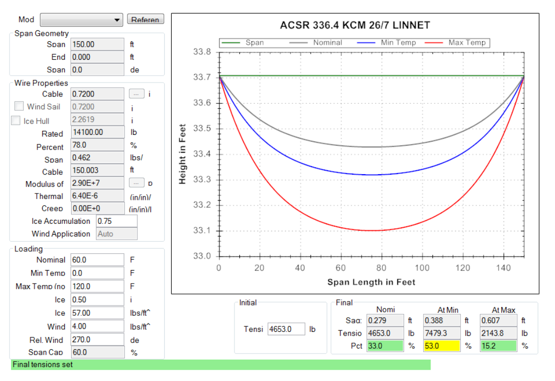
This form can also be viewed by right-clicking on a span in the inventory list and selecting “Tension of…” in the list of options. This opens up the Sag Tension Calculator. This tool can be used to view the affect of manipulating different attributes related to a particular span. Mainly a user can see what changing the default parameters will do in terms of the tension at maximum, minimum, and nominal temperatures. Each of the parameters is explained below.
Cable– Diameter of the cable
Wind Sail – The area of the cable wind load is applied to equal to the diameter times the span length
Ice Hull –
Rated – shows the rated strength of a span in lbs
Percent – The percent solid of the cable
Span – self-weight of the cable per foot length
Cable (ft) – Span of the cable
Modulus of Elasticity –
Thermal – Thermal coefficient used to determine the expansion of the cable in higher temperatures
Creep – Thermal coefficient used to determine the contraction of the cable in lower temperatures
Ice Accumulation – Defines what percentage of the cable diameter ice accumulates around
Wind Application – Wind applied is determined by the loadcase on the pole – see loadcase attributes for specific mph
Nominal – If temperature is recorded at the time of data collection, it can be entered here
Min Temp – lowest temperature considered in calculating catenary curves
Max Temp – highest temperature considered in calculating catenary curves
Ice (i) – radial ice in inches applied to the spans, as determined by the loadcase applied to a structure
Ice (lbs/ft^) – radial ice in pounds per foot
Wind (lbs/ft^) – wind speed in pounds per foot, as determined by the loadcase applied to a structure
Rel. Wind (de) – wind angle in degrees
Span Cap. (%) – maximum capacity of a span – max is always 60%
Recent Comments